Part 3: Multi-sample analysis

In this part, we are going to start from the pipeline structure we built in the previous part and extend it for multi-sample analysis.

Note

We will be working now in the multi directory. Thus, please make sure you are in the correct directory and move the data:

cd /workspaces/taxoflow_tutorial/TaxoFlow/multi
mv ../single/data .

This will give us the opportunity to practice using the following Nextflow features:

1. Using a Nextflow operator to control the flow of data
2. Controlling the execution of modules according to an input condition
3. Including a process that runs a customized script
4. Generate a performance report

---

1. Multi-sample input

With our shiny brand-new pipeline, we are at this moment able to analyze each sample individually by running the workflow multiple times. Nonetheless, one of the most powerful capabilities by Nextflow is its native parallel execution according to the available resources the executor finds. You can think of this as a sort of “integrated for loop” that will process all the samples in parallel in a single run without the need of re-running the pipeline.

Nextflow´s parallelization

Formally speaking, Nextflow’s parallelization is implicitly defined by the processes input and output declarations, or in other words, Nextflow uses asynchronous first-in, first-out (FIFO) queues or channels. If you want to know more about this, we recomend this section of the official documentation.

To achieve this purpose, there are two possibilities:

• The use of wildcards in the input (this can be tricky and requires taking into account particular folder structures).
• Create a file that points out to the sample files regardless of their location in the file system.

In this course, we will target the second input option, but you are welcome to explore how you can use the first option by checking out the Nextflow documentation.

To move forward, let’s create the file samplesheet.csv inside the folder data/:

sample_id,fastq_1,fastq_2
ERR2143768,data/samples/ERR2143768/ERR2143768_1.fastq.gz,data/samples/ERR2143768/ERR2143768_2.fastq.gz
ERR2143770,data/samples/ERR2143770/ERR2143770_1.fastq.gz,data/samples/ERR2143770/ERR2143770_2.fastq.gz
ERR2143774,data/samples/ERR2143774/ERR2143774_1.fastq.gz,data/samples/ERR2143774/ERR2143774_2.fastq.gz

Here, we have provided the sample id and the absolute paths to both forward and reverse reads per sample. Please notice that the files are not required to be stored in the directory; however, this is recommended in order to maintain a consistent fodirectorylder structure.

However, we cannot use this file as input in the current state of the pipeline, given that it expects only a path to create a paired-end channel. So let’s include an additional parameter in the multi/nextflow.config file (inside the parameter block, keeping the same structure):

sheet_csv                             = null

We initialize this parameter as null since it can be used or not.

Now, we need to modify the main.nf file to state how the input should be handled depending on the type of input:

if(params.reads){
	reads_ch = Channel.fromFilePairs(params.reads, checkIfExists:true)
} else {
	reads_ch = Channel.fromPath(params.sheet_csv)
			.splitCsv(header:true)
			.map {row-> tuple(row.sample_id, [file(row.fastq_1), file(row.fastq_2)])}
}

This modified declaration states that if we use the parameter --reads when we invoke the nextflow run main.nf, the reads channel will be created using only the path to paired-end files. Otherwise, we must include the parameter --sheet_csv with the corresponding file containing the sample information.

1.1 Conditional execution with if statements

TaxoFlow showcases two layers of conditional logic:

• At the top‑level workflow (main.nf) to decide how to build the read channel.
• Inside the TaxoFlow workflow (taxoflow.nf) to decide whether to run downstream reporting steps (shown in section 3. Conditional reporting inside taxoflow.nf).

The if statement decides how inputs are parsed:

• Branch 1 – params.reads is set:
  • Use channel.fromFilePairs(params.reads, checkIfExists:true) to build a channel of paired‑end read files directly from a glob pattern.
  • This is convenient when your reads are already organised on disk and you do not need a sample sheet.
• Branch 2 – params.reads is not set:
  • Use channel.fromPath(params.sheet_csv) followed by .splitCsv(header:true) to read a CSV samplesheet.
  • Map each row into a tuple: tuple(row.sample_id, [file(row.fastq_1), file(row.fastq_2)]).
  • This is useful when metadata such as sample_id is stored in a table.

In both cases the result is a single channel reads_ch that emits:

• A sample_id value.
• A list with the two FASTQ files.

The rest of the pipeline (TaxoFlow(...)) is independent of how reads_ch was created, illustrating a common pattern:

• Use if blocks early in the workflow to normalize different input formats into a canonical channel shape.

If structure

Abstracting the if block from main.nf:

if(condition){
    do something
} else {
    do something different
}

The else statement is not always required.

Being so, it is necessary to use one of the two forms of input; if we use both at the same time, the --reads will predominate or if none of them is indicated, the pipeline will fail. Do not worry now for the way in which channel is created using the .csv file, this declaration is quite standard and you can just copy and paste for other pipelines in which you would like to use it; however, you can learn more about this here.

Now, we would be ready to re-run the pipeline to process all the samples in a single call. Notwithstanding, the inclusion of additional samples has the advantage that we can expand the analysis to estimate β-diversity and compare them to extract important insights.

---

2. Additional processes

2.1. Kraken-biom

Let’s create a new module that is going to handle the Bracken output to produce a Biological Observation Matrix (BIOM) file that concatenates the species abundance in each sample.

The kraken_biom.nf file will be located in the multi/modules/ directory:

process KRAKEN_BIOM {
    tag "merge_samples"
    container "community.wave.seqera.io/library/kraken-biom:1.2.0--f040ab91c9691136"

    input:
    val "files"

    output:
    path "merged.biom"

    script:
    """
    list=(${files.join(' ')})
    extracted=\$(echo "\${list[@]}" | tr ' ' '\n' | awk 'NR % 3 == 2')
    kraken-biom \${extracted} --fmt json -o merged.biom
    """
    }

This process will collect each output from the Bracken files to build a single *.biom file that contains the abundance species data of all the samples. In the script statement we find three tasks to execute, the first two lines are for variable manipulation required to handle the type of input this process receives (more about this when modifying multi/taxoflow.nf below), and the second line executes the kraken-biom command that is available thanks to specified container.

2.1.1. Operator collect() and conditional execution

Nextflow provides a high number of operators that smooth data handling and orchestrates the workflow to do exactly what we want. In this case, the process KRAKEN_BIOM requires all the files produced by Bracken belonging to each sample, which means that KRAKEN_BIOM can not be triggered until all Bracken processes are finished. For this task, the operator collect() comes really handy, and therefore let’s include it in our multi/taxoflow.nf… but wait! Let’s recall that KRAKEN_BIOM and the following KNIT_PHYLOSEQ are only triggered if the execution is aiming at processing more than one sample. Being so, we will include these processes and modify the workflow execution to add the conditional statement in multi/taxoflow.nf:

include { KRAKEN_BIOM               }   from './modules/kraken_biom.nf'

if(params.sheet_csv){
	KRAKEN_BIOM(BRACKEN.out.collect())
}

Here, you can see that we have added the operator collect() to capture all the output files from BRACKEN, and this is happening only if we are using --sheet_csv as input. This operator is going to return a list of the elements specified in the output of the process (BRACKEN), and, for instance, we are interested in each “second” (indices 1,4,7…) element of the list to run the kraken-biom command; this is the reason why within the script statement in multi/modules/kraken_biom.nf we have included two codelines to obtain the paths to these files. If this is not entirely clear, please check the Nextflow documentation.

2.2. Phyloseq

2.2.1. Including a customized script

We are at the last step of the pipeline execution, and now we need to process the *.biom file by transforming it into a Phyloseq object, which is easier to use, more intuitive to understand, and is equipped with multiple tools and methods to plot. Another amazing feature by Nextflow is the possibility to run the so-called Scripts à la carte, which means that a process does not necessarily require an external tool to execute, and hence you can develop your own analysis with customized scripts, i.e., R or Python. Here, we will run an R script inside the module multi/modules/knit_phyloseq.nf to create and process the Phyloseq object taking as input the output from multi/modules/kraken_biom.nf:

process KNIT_PHYLOSEQ {
    tag "knit_phyloseq"
    container "community.wave.seqera.io/library/bioconductor-phyloseq_knit_r-base_r-ggplot2_r-rmdformats:6efceb52eb05eb44"

    input:
    path "merged"

    output:
    stdout

    script:
    def report = params.report
    def outdir = params.outdir
    """
    biom_path=\$(realpath ${merged})
    outreport=\$(realpath ${outdir})
    Rscript -e "rmarkdown::render('${report}', params=list(args='\${biom_path}'),output_file='\${outreport}/taxoReport.html')"
    """
    }

Global vs Nextflow variables

Within the modules/knit_phyloseq.nf you can notice that some variables like biom_pat and outreport are preceded by a backslash (\). In Nextflow, it is really important to distinguish Nextflow variables from Bash or environment variables. This is achieved through the use of double quotes in the script section plus adding the escape character (backslash) before Bash variables. More about this here.

As you can see, we are declaring some variables both in Nextflow and bash to be able to call the script. This is a special case since this type of scripts can be stored in the bin directory for Nextflow to find them directly. Nevertheless, as we are not “running the script” directly but we are calling Rscript to render a final *.html report, Nextflow is not able to automatically find the customized script nor detect when the report is rendered. As a result the output from this process is just a standard/command-line output, and we have to include an additional parameter in the multi/nextflow.config file:

report                             = "${projectDir}/bin/report.Rmd"

This R Markdown file uses a Phyloseq object created from Kraken2/Bracken output (BIOM file), then applies standard functions from for diversity and network analysis. Thus, results should therefore be interpreted as visual summaries of community structure, not as statistically validated differences.

Diversity and network analysis methods

Input data
Taxonomic abundance tables generated with Bracken were imported into R as a Phyloseq object. Taxa were agglomerated at the genus level (tax_glom), and low-abundance genera were filtered by retaining taxa with a mean relative abundance ≥ 3% across samples.

α-diversity (within-sample diversity)

• Calculated using plot_richness() from Phyloseq.
• Diversity indices:
  • Chao1: richness estimator accounting for unseen taxa.
  • Shannon: richness and evenness estimator.
• Normalization: raw abundance counts were used directly (no rarefaction or scaling).

β-diversity (among-sample diversity)

• Community dissimilarity calculated using Bray–Curtis distance.
• Ordination performed with Principal Coordinates Analysis (PCoA).
• Visualizations:
  • Heatmap of taxonomic abundance with sample ordering based on ordination.
  • PCoA scatter plot for comparing sample composition.
• Normalization: Bray–Curtis calculated directly from the filtered abundance table.

Network construction

• Generated using plot_net() from Phyloseq.
• Parameters:
  • Distance metric: Bray–Curtis.
  • Network type: taxa co-occurrence (type = "taxa").
  • Maximum distance threshold: maxdist = 0.9.
• Nodes represent genera; edges connect taxa based on pairwise similarity under the defined threshold.

Statistical testing

This workflow provides descriptive and exploratory analysis only. Results should therefore be interpreted as visual summaries of community structure, not as statistically validated differences. Please visit the microbiome R package tutorial for expanding the statistical analysis of microbiome data.

In addition, please notice the container used for the KNIT_PHYLOSEQ, which is combination of multiple packages required to render the *.html report. This is possible thanks to Seqera Containers, which is able to build almost any container (for docker or singularity!) by just “merging” different PyPI or Conda packages.

Also, we have to include this new process within multi/taxoflow.nf:

include { KNIT_PHYLOSEQ             }   from './modules/knit_phyloseq.nf'

We need to call it as well inside the conditional execution if multi-sample is being handled:

KNIT_PHYLOSEQ(KRAKEN_BIOM.out)

2.3. MultiQC

As noted in the method overview, the last step of the multi-sample workflow is to compile quality-control results from several tools into a single interactive report using MultiQC.

While FastQC, Trim Galore, and Kraken2 each produce their own reports per sample, MultiQC scans those outputs and builds one HTML summary that makes it easier to compare samples side by side.

Let’s create the multiqc.nf file inside the multi/modules/ directory:

process MULTIQC {
    tag "All samples"
    container "community.wave.seqera.io/library/pip_multiqc:a3c26f6199d64b7c"

    input:
    path '*'
    val output_name

    output:
    path "${output_name}.html", emit: report
    path "${output_name}_data", emit: data

    script:
    """
    multiqc . -n ${output_name}.html
    """
    }

This process runs once for the whole pipeline run, after all per-sample QC tasks have finished. Unlike the per-sample modules, its tag is fixed to "All samples" because it does not process reads from a single sample in isolation.

2.3.1. Process inputs

The input block expects two arguments:

• path '*' — a collection of report files from FastQC, Trim Galore, and Kraken2. Nextflow stages all of these files in the process work directory before the command runs.
• val output_name — the base name for the final report (in our case, this comes from params.report_id).

2.3.2. Process outputs

MultiQC produces two outputs:

• ${output_name}.html (emitted as report) — the interactive summary report you open in a browser.
• ${output_name}_data (emitted as data) — a folder with the parsed data MultiQC used to build the report.

2.3.3. Command script

The script block runs a single command: multiqc . -n ${output_name}.html. MultiQC scans the current directory (.) for recognized report formats and writes the combined HTML file. The -n flag sets the output file name.

2.3.4. Modify taxoflow.nf

First, import the new module at the top of multi/taxoflow.nf:

include { MULTIQC                     }  from './modules/multiqc.nf'

Next, we need to gather the QC files produced across all samples before calling MULTIQC. Add the following lines inside the main: block of the TaxoFlow workflow, after the per-sample processes:

multiqc_files_ch = channel.empty().mix(
FASTQC.out.zip,
FASTQC.out.html,
TRIM_GALORE.out.trimming_reports,
TRIM_GALORE.out.fastqc_reports_1,
TRIM_GALORE.out.fastqc_reports_2,
KRAKEN2.out.report,
BOWTIE2.out.log
)
multiqc_files_list = multiqc_files_ch.collect()
MULTIQC(multiqc_files_list, params.report_id)

Here is what each part does:

• channel.empty().mix(...) starts from an empty channel and merges several channels into one. Each channel contributes files from a different step: FastQC (before trimming), Trim Galore (trimming reports and post-trim FastQC), and Kraken2 (.k2report files).

Operator mix()

The mix operator combines the items emitted by two (or more) channels. More here.

• As explained before, .collect() waits until all samples have finished the upstream processes, then bundles every file into a single list. This is what allows MULTIQC to run only once, with inputs from every sample.
• MULTIQC(multiqc_files_list, params.report_id) passes that list and the report name to the process.

Unlike KRAKEN_BIOM and KNIT_PHYLOSEQ, MultiQC runs every time the pipeline runs, whether you use --reads or --sheet_csv.

Finally, expose the MultiQC outputs in the emit block:

multiqc_report           =    MULTIQC.out.report
multiqc_data             =    MULTIQC.out.data

2.3.5. Modify main.nf

We need to publish the MultiQC results in multi/main.nf, alongside the other outputs from TaxoFlow.

Add these lines to the publish block:

multiqc_report          =    TaxoFlow.out.multiqc_report
multiqc_data            =    TaxoFlow.out.multiqc_data

And assign a destination folder in the output block:

multiqc_report {
    path 'multiqc'
}
multiqc_data {
    path 'multiqc'
}

When the pipeline finishes, you will find all_samples.html (or whatever name you set in params.report_id) and the companion all_samples_data folder under output/multiqc/.

2.3.6. Parameter in nextflow.config

Add the following parameter to the params block in multi/nextflow.config:

report_id                             = "all_samples"

This value is passed to MULTIQC as the output name. You can change it at run time, for example: --report_id 'cuatro_cienegas_run'. That would produce cuatro_cienegas_run.html instead of all_samples.html.

2.3.7. Adaptation of Bowtie2

In order to include Bowtie2’s output into the final MultiQC report, we need to modify the module itself, along with additions to main.nf and taxoflow.nf:

• Changes in bowtie2.nf:

bowtie2.nf

process BOWTIE2 {
tag "${sample_id}"
container "community.wave.seqera.io/library/bowtie2:2.5.4--d51920539234bea7"

input:
tuple val(sample_id), path(read1), path(read2)
path bowtie2_index

output:
tuple val("${sample_id}"), path("${sample_id}.1"), path("${sample_id}.2"), path("${sample_id}.sam"), emit: reads
path "${sample_id}_aln_sum.log", emit: log

script:
"""
export BOWTIE2_INDEXES="${bowtie2_index}"
export index="${bowtie2_index}/\$(basename ${bowtie2_index})"
(bowtie2 -x "\${index}" -1 ${read1} -2 ${read2} -p $task.cpus -S ${sample_id}.sam --un-conc-gz ${sample_id}) 2> ${sample_id}_aln_sum.log
"""
}

Getting the stderr of Bowtie2

Bowtie2 places its output regarding the number of aligned reads to a common CLI output channel known as stderr. Thus, to capture this information we had to modify the command by using braces and create the file where we want the stderr to be stored. This file will be used by MultiQC to build the report.

• Changes in taxoflow.nf:

taxoflow.nf

workflow TaxoFlow {
// required inputs
take:
    bowtie2_index
    kraken2_db
    reads_ch
// workflow implementation
main:
     // Initial quality control
    FASTQC(reads_ch)
    TRIM_GALORE(reads_ch)
    BOWTIE2(TRIM_GALORE.out.trimmed_reads, bowtie2_index)
    KRAKEN2(BOWTIE2.out.reads, kraken2_db)
    BRACKEN(KRAKEN2.out.files, kraken2_db)
    K_REPORT_TO_KRONA(BRACKEN.out)
    KT_IMPORT_TEXT(K_REPORT_TO_KRONA.out)
    if(params.sheet_csv){
        KRAKEN_BIOM(BRACKEN.out.collect())
        KNIT_PHYLOSEQ(KRAKEN_BIOM.out)
    }
    multiqc_files_ch = channel.empty().mix(
    FASTQC.out.zip,
    FASTQC.out.html,
    TRIM_GALORE.out.trimming_reports,
    TRIM_GALORE.out.fastqc_reports_1,
    TRIM_GALORE.out.fastqc_reports_2,
    KRAKEN2.out.report
    BOWTIE2.out.log
    )
multiqc_files_list = multiqc_files_ch.collect()
MULTIQC(multiqc_files_list, params.report_id)

emit:
    bowtie_log               =    BOWTIE.out.log
    bowtie_unali             =    BOWTIE2.out.reads
    kraken_class             =    KRAKEN2.out.files
    bracken_class            =    BRACKEN.out
    krona                    =    KT_IMPORT_TEXT.out
    biom                     =    KRAKEN_BIOM.out
    fastqc_zip               =    FASTQC.out.zip
    fastqc_html              =    FASTQC.out.html
    trimmed_reads            =    TRIM_GALORE.out.trimmed_reads
    trimming_reports         =    TRIM_GALORE.out.trimming_reports
    trimming_fastqc_1        =    TRIM_GALORE.out.fastqc_reports_1
    trimming_fastqc_2        =    TRIM_GALORE.out.fastqc_reports_2
    multiqc_report           =    MULTIQC.out.report
    multiqc_data             =    MULTIQC.out.data
}

• Additions in main.nf:

main.nf

bowtie_log              =    TaxoFlow.out.bowtie_log

bowtie_log {
    path 'bowtie2'
}

---

3. Conditional reporting inside taxoflow.nf

The inner if (params.sheet_csv) in taxoflow.nf controls whether to:

• Merge Bracken outputs across samples with KRAKEN_BIOM(BRACKEN.out.collect()).
• Render a Phyloseq HTML report with KNIT_PHYLOSEQ(KRAKEN_BIOM.out).

Key ideas:

• When running from a samplesheet, we know which samples belong together, so it makes sense to aggregate them into a single biom file and downstream report.
• When running from raw file pairs only (params.reads), params.sheet_csv is null in nextflow.config, so the extra report is skipped.

This is a clean way to:

• Keep core processing always enabled.
• Toggle extra reporting or QC steps based on parameters.

---

4. Enabling the built‑in report

In nextflow.config:

report {
    enabled = true
    file = "${projectDir}/output/performanceReport.html"
}

This block tells Nextflow to:

• Generate a single HTML report named performanceReport.html at the end of each run.
• Place it in the results directory from where you launched Nextflow. Please notice that this is a custom path. It does not take from params.outdir, and thus if outdir is changed, the report will not be stored on the new output directory.
• Keep all outputs (taxonomy results, Krona plots, RMarkdown report, MultiQC output,Nextflow report) under a single output/ tree.

You do not need to change main.nf or taxoflow.nf to use this feature; it is entirely controlled by configuration.

Enabling the report as a parameter

It is possible to generate the report just by adding the parameter -with-report <file_name> when executing the pipeline. More about this here.

---

5. Execution

Now, we are completely set to run the analysis for as many samples as we would like, and we will obtain a final report depicting different metrics regarding taxonomic abundance, network analysis, and α and β-diversity. Let’s execute (please remember that we are within the multi directory):

nextflow run main.nf --sheet_csv 'data/samplesheet.csv'

On the output of the command line, you will see:

Multi-sample execution

Output

N E X T F L O W   ~  version 25.10.4

Launching `main.nf` [stoic_miescher] DSL2 - revision: 8f65b983e6

    ___________________________________________________________________________________________________
    ___________________________________________________________________________________________________
    >===>>=====>                                 >=======>  >=>                         
        >=>                                      >=>        >=>                         
        >=>        >=> >=>  >=>   >=>    >=>     >=>        >=>    >=>     >=>      >=> 
        >=>      >=>   >=>    >> >=>   >=>  >=>  >=====>    >=>  >=>  >=>   >=>  >  >=> 
        >=>     >=>    >=>     >>     >=>    >=> >=>        >=> >=>    >=>  >=> >>  >=> 
        >=>      >=>   >=>   >>  >=>   >=>  >=>  >=>        >=>  >=>  >=>   >=>>  >=>=> 
        >=>       >==>>>==> >=>   >=>    >=>     >=>       >==>    >=>     >==>    >==>     
                                                                                                    
    ___________________________________________________________________________________________________
    ___________________________________________________________________________________________________

executor >  local (24)
[1f/176196] TaxoFlow:FASTQC (ERR2143768)            [100%] 3 of 3 ✔
[c5/42b877] TaxoFlow:TRIM_GALORE (ERR2143774)       [100%] 3 of 3 ✔
[da/6ba52f] TaxoFlow:BOWTIE2 (ERR2143774)           [100%] 3 of 3 ✔
[45/054c41] TaxoFlow:KRAKEN2 (ERR2143774)           [100%] 3 of 3 ✔
[30/94f39e] TaxoFlow:BRACKEN (ERR2143774)           [100%] 3 of 3 ✔
[67/1dabc3] TaxoFlow:K_REPORT_TO_KRONA (ERR2143774) [100%] 3 of 3 ✔
[ed/8bf05a] TaxoFlow:KT_IMPORT_TEXT (ERR2143774)    [100%] 3 of 3 ✔
[b2/cfd842] TaxoFlow:KRAKEN_BIOM (merge_samples)    [100%] 1 of 1 ✔
[cb/815f36] TaxoFlow:KNIT_PHYLOSEQ (knit_phyloseq)  [100%] 1 of 1 ✔
[7f/b77259] TaxoFlow:MULTIQC (All samples)          [100%] 1 of 1 ✔

Completed at: 27-Nov-2025 13:03:40
Duration    : 1m 36s
CPU hours   : (a few seconds)
Succeeded   : 10

Use your own data

If you want to use your own data, you just need to change sample IDs and the paths to sequencing reads on the file data/samplesheet.csv, or create your own one to use it with the parameter --sheet_csv.

Keep in mind that since the execution is in parallel, the order in which the samples are processed is random and the order in which sample ids appear will differ among executions. Also, while the pipeline is running you will see that KRAKEN_BIOM, and hence KNIT_PHYLOSEQ, will not be triggered until all the samples are processed by the previous processes.

Finally, inside the output directory, you will see multiple folders with the exact sample ids, and within these all the output files, including the files to visualize the Krona plots. Likewise, in the output folder you will see the file TaxoReport.html which is ready to be opened and explored. It’s your time to analyze it!

Below you can see the plots included in the report, where it is possible to observe different metrics and general trends of annotated reads at genus level considering the custom database that we created for this tutorial with only 54 bacterial species (we applied a filter to keep only genera with relative above 3%, and keep in mind that this is the Bracken output!):

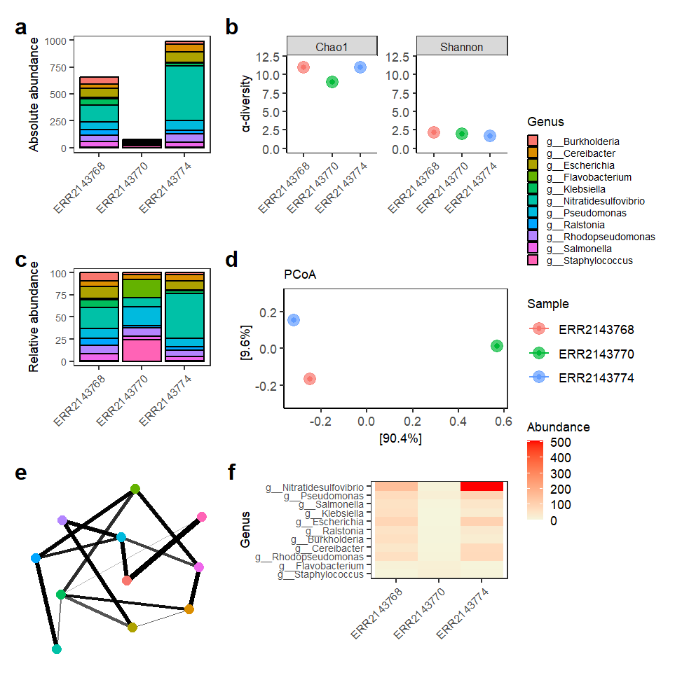
Taxonomic composition and diversity analyses of metagenomic samples. Absolute (a) and relative (c) abundance plots show the distribution of dominant genera across samples. α-diversity (b) was estimated using Chao1 and Shannon indices. β-diversity (d) was assessed by Principal Coordinates Analysis (PCoA) using Bray–Curtis distance. A co-occurrence network (e) shows relationships among genera based on Bray–Curtis similarity (maxdist = 0.9). A heatmap (f) displays genus abundance patterns across samples, ordered according to Bray–Curtis dissimilarity and PCoA. Low-abundance genera (<3% mean relative abundance) were removed before diversity and network analyses.

5.1 Performance report

Open the file performanceReport.html in a browser. You will find:

• A timeline of all tasks across processes like FASTQC, BOWTIE2, KRAKEN2, BRACKEN, etc.
• A resources table with CPU, memory and time usage per process.
• A tasks section showing how many samples were processed and how long each step took.

Plot example within the performance report.

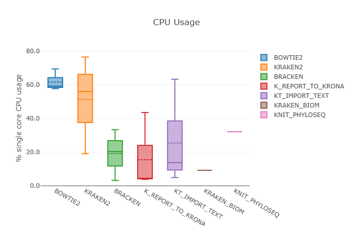
This native report complements the domain‑specific Phyloseq HTML:

• The Nextflow report focuses on pipeline performance and resource usage.
• The Phyloseq report focuses on biological interpretation of the metagenomic profiles.
• The MultiQC report focuses on general statistics and metrics aggregated from different tools.

6. Biological meaning

Once again, please remember that this execution of the pipeline, and therefore it doesn’t have a clear biological interpretation. To extract truly insights from the samples hereby provided or your own data, you need to use the corresponding genome index and Kraken2/Bracken databases for you analysis purposes. Please check how to achieve this here.

---

Takeaway

You just learnt how to control workflow execution by including conditionals and operators, processing multiple samples simultaneously and running a customized script to perform a metagenomics data analysis at read level.

What’s next?

Great! You are well equipped now to start developing your own pipelines.